library(tidyverse)Ch.16 Solutions
Prerequisites:
16.3.1 Exercises:
The two things I didn’t like about the default plot is the crowded x-axis labeling and the inclusion of multiple null options. While NAs definitely have importance in any statistical and exploratory work, for a “pretty” graph I prefer to remove them.
gss_cat |>
  ggplot(aes(x = rincome)) +
  geom_bar()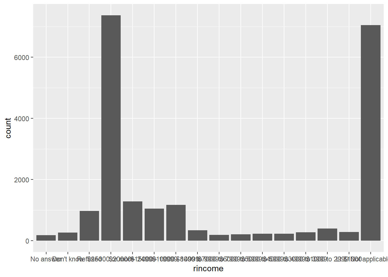
gss_cat |>
  filter(str_detect(rincome, '\\$')) |>
  ggplot(aes(y = rincome)) +
  geom_bar()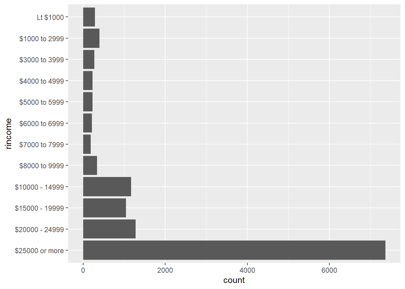
I did this through the count function. Can use an expression like
filter(n == max(n))if you only want the single largest count.gss_cat |> count(relig, sort = TRUE) ## # A tibble: 15 × 2 ## relig n ## <fct> <int> ## 1 Protestant 10846 ## 2 Catholic 5124 ## 3 None 3523 ## 4 Christian 689 ## 5 Jewish 388 ## 6 Other 224 ## 7 Buddhism 147 ## 8 Inter-nondenominational 109 ## 9 Moslem/islam 104 ## 10 Orthodox-christian 95 ## 11 No answer 93 ## 12 Hinduism 71 ## 13 Other eastern 32 ## 14 Native american 23 ## 15 Don't know 15 gss_cat |> count(partyid, sort = TRUE) ## # A tibble: 10 × 2 ## partyid n ## <fct> <int> ## 1 Independent 4119 ## 2 Not str democrat 3690 ## 3 Strong democrat 3490 ## 4 Not str republican 3032 ## 5 Ind,near dem 2499 ## 6 Strong republican 2314 ## 7 Ind,near rep 1791 ## 8 Other party 393 ## 9 No answer 154 ## 10 Don't know 1I did this by finding the number of distinct denominations options that have appeared for each religion.
gss_cat |>
  group_by(relig) |>
  summarize(distinct_relig = n_distinct(denom)) |>
  arrange(desc(distinct_relig))
## # A tibble: 15 × 2
##    relig                   distinct_relig
##    <fct>                            <int>
##  1 Protestant                          29
##  2 Christian                            4
##  3 Other                                2
##  4 No answer                            1
##  5 Don't know                           1
##  6 Inter-nondenominational              1
##  7 Native american                      1
##  8 Orthodox-christian                   1
##  9 Moslem/islam                         1
## 10 Other eastern                        1
## 11 Hinduism                             1
## 12 Buddhism                             1
## 13 None                                 1
## 14 Jewish                               1
## 15 Catholic                             1
gss_cat |> group_by(relig) |> summarize(distinct = n_distinct(denom)) |> ggplot(aes(y = relig, x = distinct)) + geom_bar(stat = 'identity')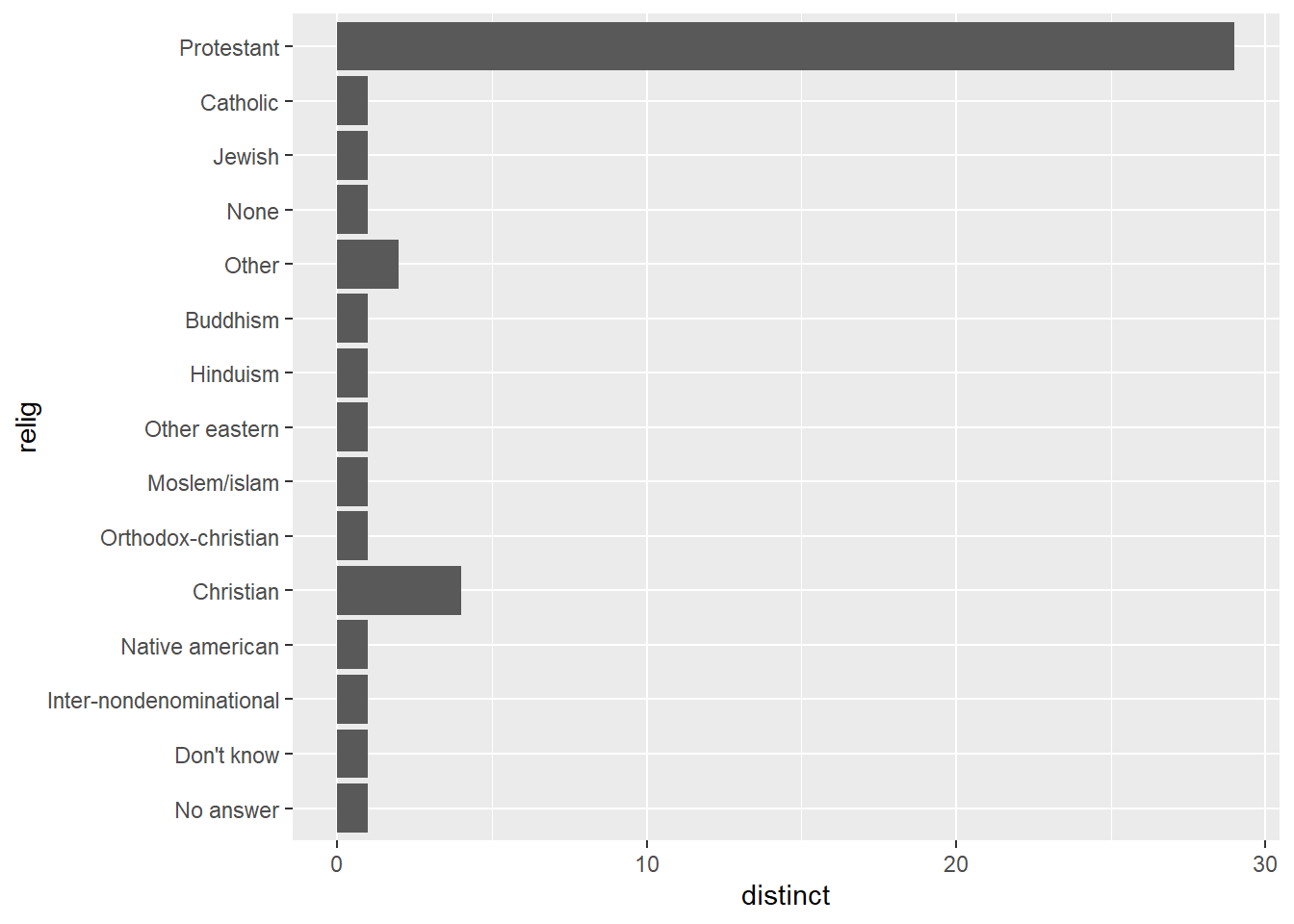
- Further analysis will show you that only protestant has specific denominations listed, since Christian and Other only have quasi-variations of null.
16.4.1 Exercises:
While median is immune to skew and worth comparing to mean to help show said skew, it’s important to realize that skew is something not to be eliminated but a characteristic of your data set worth understanding before you perform transformations of the data. Personally, while I think values above 20 tvhours are almost certainly outliers, mean is still a valuable summary statistic to me since it helps me be alert to potential skew (since it is so different than median) before I ever run a test of skewness.
gss_cat |>
  filter(!is.na(tvhours)) |>
  ggplot(aes(tvhours)) +
  geom_histogram(binwidth = 1)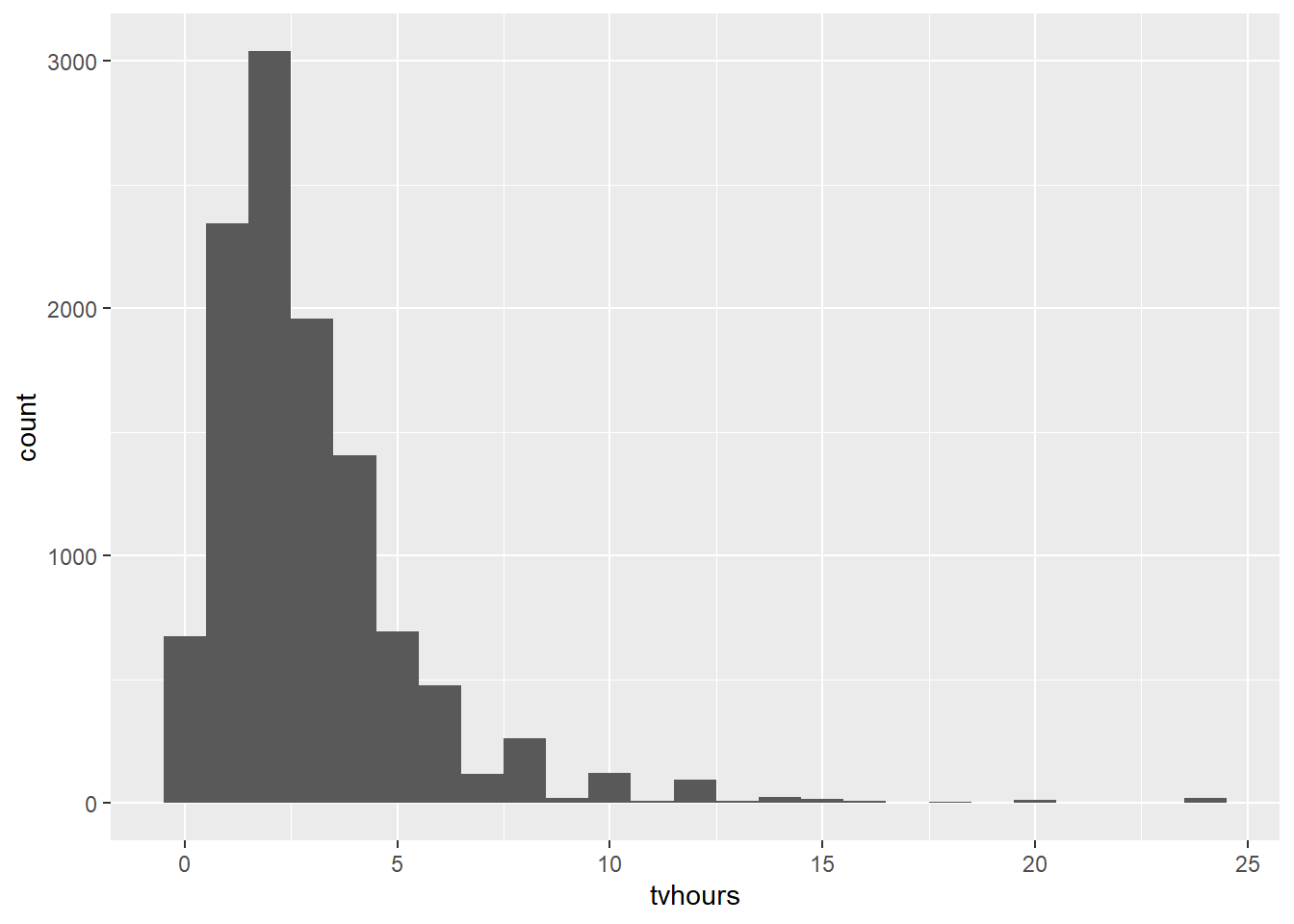
print(mean(gss_cat$tvhours, na.rm = TRUE))
## [1] 2.980771

print(median(gss_cat$tvhours, na.rm = TRUE))
## [1] 2
Included my notes after each function call.
levels(gss_cat$marital)
## [1] "No answer"     "Never married" "Separated"     "Divorced"
## [5] "Widowed"       "Married"
#Marital: Seems pretty arbitrary.

levels(gss_cat$race)
## [1] "Other"          "Black"          "White"          "Not applicable"
#race: seems pretty arbitrary.

levels(gss_cat$rincome)
##  [1] "No answer"      "Don't know"     "Refused"        "$25000 or more"
##  [5] "$20000 - 24999" "$15000 - 19999" "$10000 - 14999" "$8000 to 9999"
##  [9] "$7000 to 7999"  "$6000 to 6999"  "$5000 to 5999"  "$4000 to 4999"
## [13] "$3000 to 3999"  "$1000 to 2999"  "Lt $1000"       "Not applicable"
#Income levels are ordered sensibly. I think it's principled.

levels(gss_cat$partyid)
##  [1] "No answer"          "Don't know"         "Other party"
##  [4] "Strong republican"  "Not str republican" "Ind,near rep"
##  [7] "Independent"        "Ind,near dem"       "Not str democrat"
## [10] "Strong democrat"
#partyid is ordered from right to left wing. principled.

levels(gss_cat$relig)
##  [1] "No answer"               "Don't know"
##  [3] "Inter-nondenominational" "Native american"
##  [5] "Christian"               "Orthodox-christian"
##  [7] "Moslem/islam"            "Other eastern"
##  [9] "Hinduism"                "Buddhism"
## [11] "Other"                   "None"
## [13] "Jewish"                  "Catholic"
## [15] "Protestant"              "Not applicable"
#relig seems pretty abitrary.

levels(gss_cat$denom)
##  [1] "No answer"            "Don't know"           "No denomination"
##  [4] "Other"                "Episcopal"            "Presbyterian-dk wh"
##  [7] "Presbyterian, merged" "Other presbyterian"   "United pres ch in us"
## [10] "Presbyterian c in us" "Lutheran-dk which"    "Evangelical luth"
## [13] "Other lutheran"       "Wi evan luth synod"   "Lutheran-mo synod"
## [16] "Luth ch in america"   "Am lutheran"          "Methodist-dk which"
## [19] "Other methodist"      "United methodist"     "Afr meth ep zion"
## [22] "Afr meth episcopal"   "Baptist-dk which"     "Other baptists"
## [25] "Southern baptist"     "Nat bapt conv usa"    "Nat bapt conv of am"
## [28] "Am bapt ch in usa"    "Am baptist asso"      "Not applicable"
#denom seems pretty abitrary.
Its because having x as numeric and y as the categorical variable is analogous to flipping the coordinates around the origin from a plot with x as the categorical and y as the numeric. Therefore the y-axis is “counting up” as you move up vertically and the first position is the one closes to the origin.
16.5.1 Exercises:
I decided to group many factor levels together to simplify my graph. Granted, this is not without issues since you can justifiably categorize a value like “Ind,near dem” as either democrat or independent.
gss_cat |>
  mutate(
    partyid = fct_collapse(partyid,
      "other" = c("No answer", "Don't know", "Other party"),
      "rep" = c("Strong republican", "Not str republican"),
      "ind" = c("Ind,near rep", "Independent", "Ind,near dem"),
      "dem" = c("Not str democrat", "Strong democrat")
    )
  ) |>
  group_by(year, partyid) |>
  summarise(n = n()) |>
  mutate(prop = n / sum(n)) |>
  ggplot(aes(year, prop, color = partyid)) +
  geom_smooth(se = FALSE)
## `summarise()` has grouped output by 'year'. You can override using the
## `.groups` argument.
## `geom_smooth()` using method = 'loess' and formula = 'y ~ x'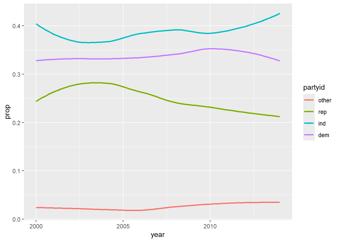
I decided to create $5000 partitions.
gss_cat |> mutate( rincome = fct_collapse(rincome, '0-5k' = c('Lt $1000', '$1000 to 2999', '$3000 to 3999', '$4000 to 4999'), '5-10k' = c('$5000 to 5999', '$6000 to 6999', '$7000 to 7999', '$8000 to 9999'))) |> distinct(rincome) ## # A tibble: 10 × 1 ## rincome ## <fct> ## 1 5-10k ## 2 Not applicable ## 3 $20000 - 24999 ## 4 $25000 or more ## 5 $10000 - 14999 ## 6 Refused ## 7 $15000 - 19999 ## 8 0-5k ## 9 Don't know ## 10 No answerfct_lump()will roll uncommon values into Other by default, and since that is already a top 10 value in relig, there is no need to create an 11th option. If you change the name of “Other” you then get 11th factor levels (including Other).gss_cat |> count(relig, sort = TRUE) ## # A tibble: 15 × 2 ## relig n ## <fct> <int> ## 1 Protestant 10846 ## 2 Catholic 5124 ## 3 None 3523 ## 4 Christian 689 ## 5 Jewish 388 ## 6 Other 224 ## 7 Buddhism 147 ## 8 Inter-nondenominational 109 ## 9 Moslem/islam 104 ## 10 Orthodox-christian 95 ## 11 No answer 93 ## 12 Hinduism 71 ## 13 Other eastern 32 ## 14 Native american 23 ## 15 Don't know 15 gss_cat |> mutate(relig = fct_lump_n(relig, n = 10)) |> count(relig, sort = TRUE) ## # A tibble: 10 × 2 ## relig n ## <fct> <int> ## 1 Protestant 10846 ## 2 Catholic 5124 ## 3 None 3523 ## 4 Christian 689 ## 5 Other 458 ## 6 Jewish 388 ## 7 Buddhism 147 ## 8 Inter-nondenominational 109 ## 9 Moslem/islam 104 ## 10 Orthodox-christian 95 gss_cat |> mutate(relig = fct_recode(relig, 'other' = 'Other' )) |> mutate(relig = fct_lump_n(relig, n = 10)) |> count(relig, sort = TRUE) ## # A tibble: 11 × 2 ## relig n ## <fct> <int> ## 1 Protestant 10846 ## 2 Catholic 5124 ## 3 None 3523 ## 4 Christian 689 ## 5 Jewish 388 ## 6 Other 234 ## 7 other 224 ## 8 Buddhism 147 ## 9 Inter-nondenominational 109 ## 10 Moslem/islam 104 ## 11 Orthodox-christian 95