ch_17_solutions

Prerequisites:

library(tidyverse)
library(nycflights13)

17.2.5 Exercises:

Returns an NA value and gives a warning message with the number of elements to fail.
It determines the timezone to be used when returning the date. By default it will use your computer system’s timezone.

Code below.

d1 <- "January 1, 2010"
parse_date(d1, '%B %d, %Y')
## [1] "2010-01-01"
mdy(d1)
## [1] "2010-01-01"

d2 <- "2015-Mar-07"
parse_date(d2, '%Y-%b-%e')
## [1] "2015-03-07"
ymd(d2)
## [1] "2015-03-07"

d3 <- "06-Jun-2017"
parse_date(d3, '%e-%b-%Y')
## [1] "2017-06-06"
dmy(d3)
## [1] "2017-06-06"

d4 <- c("August 19 (2015)", "July 1 (2015)")
parse_date(d4, '%B %d (%Y)')
## [1] "2015-08-19" "2015-07-01"
mdy(d4)
## [1] "2015-08-19" "2015-07-01"

d5 <- "12/30/14" # Dec 30, 2014
parse_date(d5, '%m/%e/%y')
## [1] "2014-12-30"
mdy(d5)
## [1] "2014-12-30"

t1 <- "1705"
parse_time(t1, '%H%M')
## 17:05:00
hm(paste0(substr(t1, 1, 2), ':', substr(t1, 3, 5)))
## [1] "17H 5M 0S"
#had trouble using lubridate w/o modifying the string to include a colon.

t2 <- "11:15:10.12 PM"
parse_time(t2, '%I:%M:%OS %p')
## 23:15:10.12
hms(t2)
## [1] "11H 15M 10.12S"

17.3.4 Exercises:

For these exercises I used a modified version of the flights_dt data set used throughout the chapter. As partially discussed in section 17.4.2, the year, month, day component of flights refers only to the day of departure and not the schedule date nor the arrival date so I created a data set using periods and the delays to circumvent that issue.

make_datetime_100 <- function(year, month, day, time) {
  make_datetime(year, month, day, time %/% 100, time %% 100)
}

flights <- flights |> 
  mutate(id = row_number())

flights_datetime <- flights |> 
  filter(!is.na(dep_time), !is.na(arr_time)) |> 
  mutate(
    dep_time = make_datetime_100(year, month, day, dep_time),
    arr_time = if_else(make_datetime_100(year, month, day, arr_time) < dep_time,  
                       make_datetime_100(year, month, day, arr_time) + days(1),
                       make_datetime_100(year, month, day, arr_time)),
    sched_dep_time = dep_time - minutes(dep_delay),
    sched_arr_time = arr_time - minutes(arr_delay)
  )

To confirm the accuracy of my transformations, I pull the HHMM of my modified arr_time, sched_dep_time and sched_arr_time times to see if it matched the original values. A weird quirk I found is that flights listed midnight as 2400 as opposed to 0, hence the modular divisor I used in my filter below.

flights_datetime |> 
  inner_join(flights, by = join_by('id')) |> 
  filter(
    ((hour(arr_time.x) * 100 + minute(arr_time.x)) != arr_time.y %% 2400) |
    ((hour(sched_dep_time.x) * 100 + minute(sched_dep_time.x)) != sched_dep_time.y %% 2400) |
    ((hour(sched_arr_time.x) * 100 + minute(sched_arr_time.x)) != sched_arr_time.y %% 2400) 
  )
## # A tibble: 0 × 39
## # ℹ 39 variables: year.x <int>, month.x <int>, day.x <int>, dep_time.x <dttm>,
## #   sched_dep_time.x <dttm>, dep_delay.x <dbl>, arr_time.x <dttm>,
## #   sched_arr_time.x <dttm>, arr_delay.x <dbl>, carrier.x <chr>,
## #   flight.x <int>, tailnum.x <chr>, origin.x <chr>, dest.x <chr>,
## #   air_time.x <dbl>, distance.x <dbl>, hour.x <dbl>, minute.x <dbl>,
## #   time_hour.x <dttm>, id <int>, year.y <int>, month.y <int>, day.y <int>,
## #   dep_time.y <int>, sched_dep_time.y <int>, dep_delay.y <dbl>, …

Lots of ways to approach this question, I decided to create a frequency plot split by quarter to see if there was a visual trend. While I didn’t find anything apparent, some candidates for future analysis:
- See if there is a difference in a month-by-month or week-by-week grouping. Going to be a noisy plot, but setting an alpha-level to the plot or just viewing the distribution of summary statistics (mean etc.) might make it more manageable.
- See if the mean flight time changes over the course of the year.
```
flights_datetime |> 
  mutate(
    dep_hour = hms::as_hms(dep_time - floor_date(dep_time, "day")),
    dep_quarter = as.character(quarter(dep_time))
  ) |> 
  ggplot(aes(x = dep_hour, color = dep_quarter)) +
  geom_freqpoly(binwidth = 60 * 30)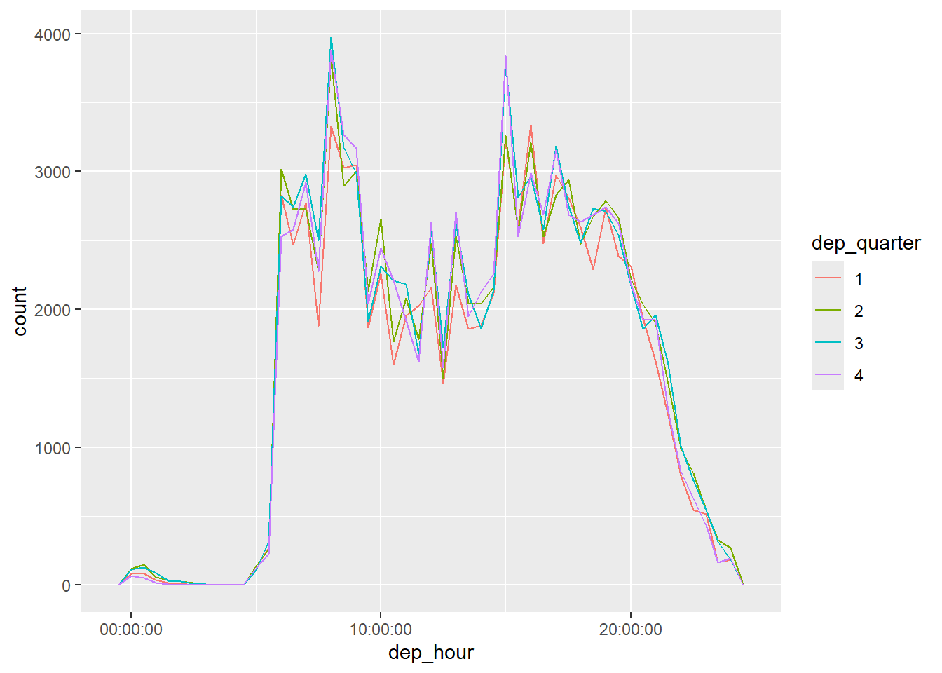
```

I somewhat tested this earlier when I confirmed my flights_ datetime data set matches the original data set.

make_datetime_100 <- function(year, month, day, time) {
  make_datetime(year, month, day, time %/% 100, time %% 100)
}

flights_datetime |> 
  filter(dep_time - sched_dep_time != minutes(dep_delay))
## # A tibble: 0 × 20
## # ℹ 20 variables: year <int>, month <int>, day <int>, dep_time <dttm>,
## #   sched_dep_time <dttm>, dep_delay <dbl>, arr_time <dttm>,
## #   sched_arr_time <dttm>, arr_delay <dbl>, carrier <chr>, flight <int>,
## #   tailnum <chr>, origin <chr>, dest <chr>, air_time <dbl>, distance <dbl>,
## #   hour <dbl>, minute <dbl>, time_hour <dttm>, id <int>

flights_datetime |> 
  mutate(diff = dep_time - sched_dep_time)
## # A tibble: 328,063 × 21
##     year month   day dep_time            sched_dep_time      dep_delay
##    <int> <int> <int> <dttm>              <dttm>                  <dbl>
##  1  2013     1     1 2013-01-01 05:17:00 2013-01-01 05:15:00         2
##  2  2013     1     1 2013-01-01 05:33:00 2013-01-01 05:29:00         4
##  3  2013     1     1 2013-01-01 05:42:00 2013-01-01 05:40:00         2
##  4  2013     1     1 2013-01-01 05:44:00 2013-01-01 05:45:00        -1
##  5  2013     1     1 2013-01-01 05:54:00 2013-01-01 06:00:00        -6
##  6  2013     1     1 2013-01-01 05:54:00 2013-01-01 05:58:00        -4
##  7  2013     1     1 2013-01-01 05:55:00 2013-01-01 06:00:00        -5
##  8  2013     1     1 2013-01-01 05:57:00 2013-01-01 06:00:00        -3
##  9  2013     1     1 2013-01-01 05:57:00 2013-01-01 06:00:00        -3
## 10  2013     1     1 2013-01-01 05:58:00 2013-01-01 06:00:00        -2
## # ℹ 328,053 more rows
## # ℹ 15 more variables: arr_time <dttm>, sched_arr_time <dttm>, arr_delay <dbl>,
## #   carrier <chr>, flight <int>, tailnum <chr>, origin <chr>, dest <chr>,
## #   air_time <dbl>, distance <dbl>, hour <dbl>, minute <dbl>, time_hour <dttm>,
## #   id <int>, diff <drtn>

Code below:

flights_datetime |> 
  mutate(
    dep_arr_diff = as.duration(arr_time -  dep_time),
    air_time = dminutes(air_time)
  ) |> 
  select(dep_time, arr_time, dep_arr_diff, air_time)
## # A tibble: 328,063 × 4
##    dep_time            arr_time            dep_arr_diff        
##    <dttm>              <dttm>              <Duration>          
##  1 2013-01-01 05:17:00 2013-01-01 08:30:00 11580s (~3.22 hours)
##  2 2013-01-01 05:33:00 2013-01-01 08:50:00 11820s (~3.28 hours)
##  3 2013-01-01 05:42:00 2013-01-01 09:23:00 13260s (~3.68 hours)
##  4 2013-01-01 05:44:00 2013-01-01 10:04:00 15600s (~4.33 hours)
##  5 2013-01-01 05:54:00 2013-01-01 08:12:00 8280s (~2.3 hours)  
##  6 2013-01-01 05:54:00 2013-01-01 07:40:00 6360s (~1.77 hours) 
##  7 2013-01-01 05:55:00 2013-01-01 09:13:00 11880s (~3.3 hours) 
##  8 2013-01-01 05:57:00 2013-01-01 07:09:00 4320s (~1.2 hours)  
##  9 2013-01-01 05:57:00 2013-01-01 08:38:00 9660s (~2.68 hours) 
## 10 2013-01-01 05:58:00 2013-01-01 07:53:00 6900s (~1.92 hours) 
## # ℹ 328,053 more rows
## # ℹ 1 more variable: air_time <Duration>

Airtime can be greater than or less than the difference between departure time and arrival time, this isn’t an error since flights across time zones will have an effect on timestamps but not the length of time spent in the air.

I would use sched_dep_time since that is when the delay starts.

flights_datetime |> 
  mutate(
    dep_hour = hms::as_hms(sched_dep_time - floor_date(sched_dep_time, "day"))
  ) |>
  ggplot(aes(x = dep_hour, y = dep_delay)) +
  geom_smooth()
## `geom_smooth()` using method = 'gam' and formula = 'y ~ s(x, bs = "cs")'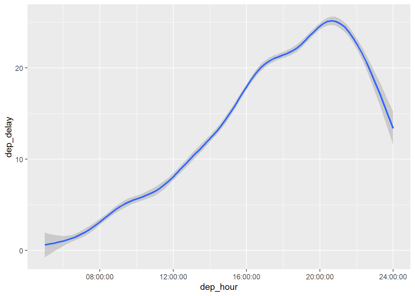

Since we are looking at only 7 options, I personally find a table more readable.

flights_datetime |> 
  mutate(wday = wday(dep_time, label = TRUE)) |> 
  group_by(wday) |> 
  summarize(
    prop_delay = mean(dep_delay > 0),
    total_flights = n()
  )
## # A tibble: 7 × 3
##   wday  prop_delay total_flights
##   <ord>      <dbl>         <int>
## 1 Sun        0.383         45583
## 2 Mon        0.401         49396
## 3 Tue        0.364         49226
## 4 Wed        0.372         48753
## 5 Thu        0.431         48565
## 6 Fri        0.425         48645
## 7 Sat        0.348         37895

To minimize the chance of any delay, Saturday looks best (also notice that it has less flights than the other days). As an extension of this problem, you may want to see the average delay by day and the chance of a severe delay.

Both have an increased frequency at round numbers. Can look at Section 10.3.1 and 17.3.1 of the book to see examples of a similar trend in the diamonds and flights dataset respectively.

My plot shows that flights that were delayed are more uniform across the hour while flights that left early are more likely to leave early between the 20-30 and 50-60 minute range.

flights_datetime |> 
  mutate(
    delayed = if_else(dep_delay>0, TRUE,FALSE),
    dep_minute = minute(hms::as_hms((dep_time - floor_date(dep_time, "hour"))))
  )|> 
  ggplot(aes(dep_minute))+
  geom_histogram(bins = 60) +
  facet_wrap(~delayed) +
  labs(title = 'Plot faceted by if dep_delay > 0')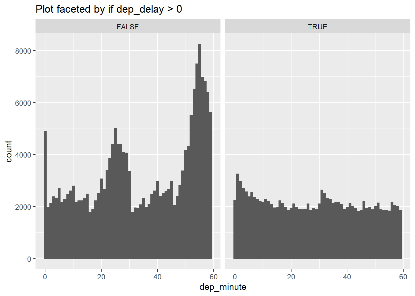

17.4.4:

Logical vectors will automatically be coerced to a 1 (TRUE) or 0 (FALSE) if a numerical value is expected. Therefore days(overnight) will return days(0) if FALSE or days(1) if TRUE.

Notice I start with month 0 to make sure I include the original date.

first_day <- ymd('2015-01-01')
first_day + months(0:11)
##  [1] "2015-01-01" "2015-02-01" "2015-03-01" "2015-04-01" "2015-05-01"
##  [6] "2015-06-01" "2015-07-01" "2015-08-01" "2015-09-01" "2015-10-01"
## [11] "2015-11-01" "2015-12-01"

floor_date(today(), 'year') + months(0:11)
##  [1] "2025-01-01" "2025-02-01" "2025-03-01" "2025-04-01" "2025-05-01"
##  [6] "2025-06-01" "2025-07-01" "2025-08-01" "2025-09-01" "2025-10-01"
## [11] "2025-11-01" "2025-12-01"

I made sure to use an interval for this problem even though I admittedly had trouble thinking of a specific scenario where a duration-based function would give a different result.

birthday_function <- function(birthday) {
  (birthday %--% today()) %/% years(1)
}
birthday_function(ymd('2023-07-07 00:00:00'))
## Warning: All formats failed to parse. No formats found.
## [1] NA

While the expression does work without error most of the time, the numerator doesn’t work since adding a year returns null if the date created is invalid (such as in leap years).
```
(today() %--% (today() + years(1))) / months(1)
## [1] 12
(as_date('2024-02-29') %--% (as_date('2024-02-29') + years(1))) %/% months(1)
## [1] NA
```
- Also, reading the vignette here, you can see it’s recommended to use integer division since the result is more intuitive.
```
(as_date('2024-02-28') %--% (as_date('2024-02-28') + years(1))) %/% months(1)
## [1] 12
```